Note on reciprocal Bernoulli probability estimation

Tossing a coin for heads or tails constitutes a Bernoulli trial. A random variable follows a Bernoulli distribution if there are two possible outcomes: one of the outcomes ("success") occurring with probability $p$, and– consequently –the other outcome ("failure") occurring with probability $1-p$ (often denoted $q$).

Given the ability to repeatedly sample from the Bernoulli experiment (toss the coin a bunch and record outcomes), it is well-known and well-studied how to estimate $p$ to a certain additive precision. Simply toss the coin $n=3/(2{ϵ}^2)$ times, and estimate $p$ as

$$\hat{p}=\frac{\text{number of successes}}{n}$$

which is to say, $p$ is estimated as the fraction of observed successes in the number of taken trials. Why is this sufficient? The Chebyshev inequality states that, for any random variable $X$ with non-zero variance $𝐕X$ and mean $𝐄X$,

$$𝐏[|X-𝐄X|\ge ϵ]\le \frac{𝐕X}{{ϵ}^2}.$$

Since the number of successes out of $n$ trials follows (by definition) a Binomial distribution, then one finds that

$$𝐄\hat{p}=p$$ $$𝐕\hat{p}=\frac{p(1-p)}{n}$$

from whence, and using the Chebyshev bound, one finds the following statement:

$$𝐏[|\hat{p}-p|\ge ϵ]\le \frac{p(1-p)}{n{ϵ}^2}.$$

Since $p\in [0,1]$, $p(1-p)\in [0,1/2]$, it follows that setting $n=3/(2{ϵ}^2)$, as proposed, ensures a success probability of our estimation of $2/3$. (This can be improved to arbitrary success with a technique called median of means, which I will not discuss here.)

Therefore, consider now the similar problem of estimating $1/p$: given the ability to sample from $B~\text{Bernoulli}(p)$, can you estimate $1/p$ to additive precision $ϵ$? (With success probability at least $2/3$.) The answer seems to be surprisingly hard, if you want a proof.¹

Dagum, Karp, Luby, Ross (2000) use a neat trick to construct a random variable whose mean is $1/p$. The trick is as follows: toss the coin until you see a success, counting the number of tosses. Let $G$ be the random variable corresponding to the number of tosses. By definition, $G$ follows a geometric distribution. Now, prepare $G$ independent copies of $A$, a random variable following an exponential distribution of rate $\lambda =1$. (This is something your computer will happily do for you.) Let these copies be $A_1,A_2,\dots ,A_G$. If you add these up, you can show² that

$$S=A_1+A_2+\cdots +A_G~\text{Exp}(p).$$

I.e., $S$ is an exponential distribution with rate $p$! Therefore it has properties

$$𝐄S=\frac{1}{p}$$ $$𝐕S=\frac{1}{p^2}.$$

It follows that $S$ is an unbiased estimator for $1/p$ – only it has pretty poor variance. If you average out $k$ i.i.d. copies of $S$ – call that ${\bar{S}}_k$, – then³

$$𝐄{\bar{S}}_k=\frac{1}{p}$$ $$𝐕{\bar{S}}_k=\frac{1}{k{p}^2}.$$

To make sure your needed number of copies does not scale with $p$– in other words, with the parameter you’re trying to estimate itself –the variance should be (bounded by a) constant. (Cf. the discussion of the Chebyshev inequality above.) This is not the case for ${\bar{S}}_k$. Another way to look at this is to apply the Chebyshev inequality directly to ${\bar{S}}_k$, to find

$$𝐏[|{\bar{S}}_k-\frac{1}{p}|\ge ϵ]\le \frac{1}{ϵk{p}^2}.$$

There’s no way to find a $k$ that bounds the right-hand side to $1/3$ without knowledge of $p$.

An idea is to choose $k$ itself based on sampling from the Bernoulli experiment. Why? We know that $k$ should be bigger the smaller $p$ is. And, we know that if $G$ follows a geometric distribution with rate $p$, then smaller $p$ yields larger values of $G$; under expectation, $G=1/p$. Then, maybe, ${\bar{S}}_{G^2}$ has constant variance?

Surprisingly, not at all: following something like a conditional Monte Carlo technique⁴, we can calculate the mean and variance as follows:

$$𝐄[{\bar{S}}_{G^2}]={𝐄}_G[{𝐄}_S[{\bar{S}}_{g^2}|G=g]]=\frac{1}{p}$$ $$𝐕[{\bar{S}}_{G^2}]=𝐄[({\bar{S}}_{G^2}{)}^2]-\frac{1}{p^2}=\frac{1}{p^2}𝐄[\frac{1}{G^2}]$$

This expected value can be explicitly computed with the knowledge of the PDF of a geometric variable with rate $p$:

$$𝐄[\frac{1}{G^2}]={\sum }_{n=1}^{\infty }\frac{1}{n^2}(1-p{)}^{n-1}p=\frac{p}{1-p}{\text{Li}}_2(1-p).$$

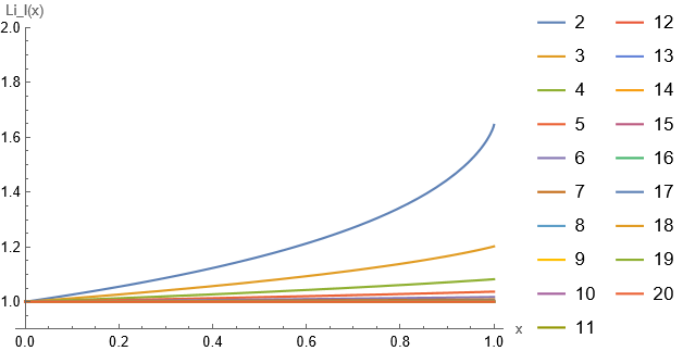
${\text{Li}}_2(x)$ denotes the "dilogarithm function"; it is the special $l=2$ case of the polylogarithm function family:

$${\text{Li}}_l(x)={\sum }_{n=1}^{\infty }\frac{x^n}{n^l}.$$

Therefore, we conclude that the variance of ${\bar{S}}_{G^2}$ is

$$𝐕{\bar{S}}_{G^2}=\frac{{\text{Li}}_2(1-p)}{p(1-p)}$$

You can find, graphically, that ${\text{Li}}_2(x)/x$ is bounded from above and below by constants (specifically, $1.8$ and $1$, respectively), so the variance here is still of the order of $1/p$.

What if we take an even greater power of $G~\text{Geo}(p)$?

Unfortunately, everything follows very similarly to as before, resulting in a variance of

$$𝐕{\bar{S}}_{G^l}=\frac{{\text{Li}}_l(1-p)}{p(1-p)}.$$

Indeed, ${\text{Li}}_l(x)$ is seems to be bounded from above and below for any value of $l$:

Therefore the variance of such an estimator will always be of the order $1/p$.

Is it possible to provably estimate inverse of Bernoulli probabilities to constant precision at all?